Estimated Time

This lesson should take approximately 1 hour and 30 min to cover and watch all the video material. Make sure you have R Studio open to work through the examples provided!

Required viewing

There are two prescribed videos before you start this lesson.

The below video is 20min long and covers the R Studio environment, customising R Studio and the first operator called leftward assignment. Please note that there are time stamps in if you watch the video in Loom.

The second video is 15min long and covers objects and object assignment and some basic of indexing (which we go over in more detail in this document). Again time stamped video here

Visualising a vector

A vector (referring here to atomic vectors) is a one dimensional object (it only has length) that can store only one type of data (you can’t mix numbers and strings). This data type could be any one of the following:

String (this contains data like words or letters)
Numeric or Double (these are numbers)
Logical (these are TRUE or FALSE and can be abbreviated to T and F)
Factor (a special data type used for categories)

Let’s create a vector in R and visualise it.

Vec_1 <- c("A", "B", "C", "D", "E")

Notice that we use the leftward assignment operator “<-” to assign the data and the “c()” function to combine each element we want to assign. Also notice that we use the “,” to separate which data goes into which element.

If we want to see what’s inside our newly created vector we could do the following:

Vec_1

[1] "A" "B" "C" "D" "E"

Or:

View(Vec_1)

Note the capital “V” in View (R is case-sensitive).

View will bring up a new window to view your object in R Studio.

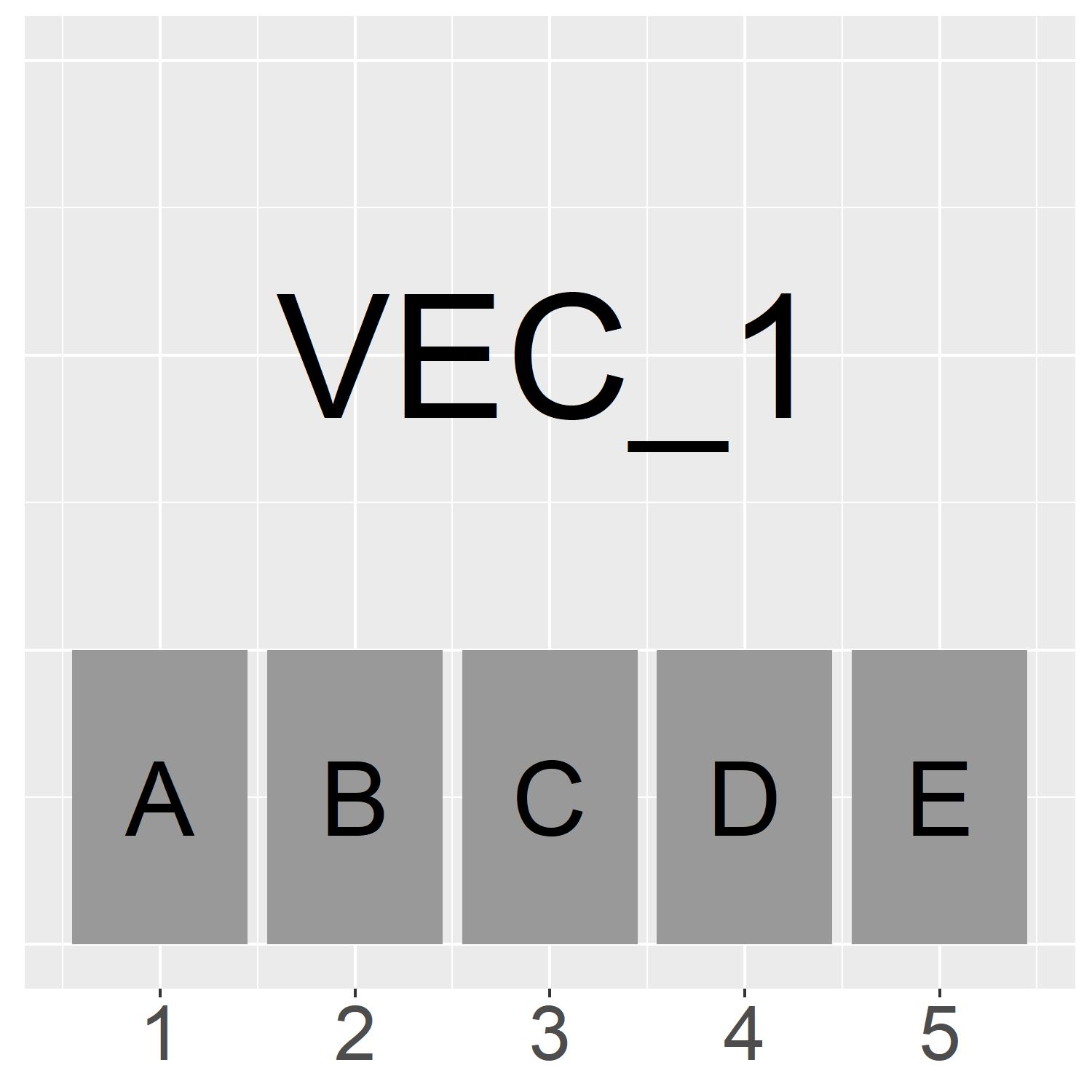
On the left is a visualisation of the vector we just created called “Vec_1”.
The vector has a length of 5 and it is a “character” vector.
This means it can contains “string” variables inside of it. We can see the first 5 letters of the alphabet are stored in each element of the vector
A brief explanation and some rules about strings can be found here.
The structure of this vector can be represented as:

\[\LARGE Vec\_1[1:5]\]

Indexing a vector

Next, we may want to extract some of the information stored inside of the vector.

In this case, the vector contains letters A, B, C, D and E.

The GIF on the left shows what command we would use to access each element of the vector
As our index goes from 1 to 5, we can access the information stored in each element
Because the information stored are strings, they are returned with "" around them
The general rule to index a vector is: \[\Large Vec\_1[element]\]
Note that we can select more than one element of a vector at a time such as elements 2 and 4 (you’ll see in the matrix section why we can’t just type Vec_1[2, 4]): \[\Large Vec\_1[c(2, 4)]\]
Or all elements in a range such as elements 2, 3 and 4: \[\Large Vec\_1[2:4]\]

Play around with each of the above vector indexing methods and make sure you understand how they work. Also think about what would happen if you introduce a “-” operator?

Visualising a matrix

A matrix is a two-dimensional object that has both rows and columns. Similar to the vector above, it can also only store one type of data.

Let’s create a matrix similar to the vector we created above. But because its a 2 dimensional object we can give it 5 rows and 5 columns.

This means it will have space for 25 letters of the alphabet instead of just 5.

But first, I don’t want to have to type out all the letters from “A” to “Y” so we will introduce the built in vector “LETTERS”. “LETTERS” is a vector of all letters in the alphabet. You can also use “letters” if you want lower case letters.

LETTERS

 [1] "A" "B" "C" "D" "E" "F" "G" "H" "I" "J" "K" "L" "M" "N" "O" "P" "Q" "R" "S" "T" "U" "V"
[23] "W" "X" "Y" "Z"

letters

 [1] "a" "b" "c" "d" "e" "f" "g" "h" "i" "j" "k" "l" "m" "n" "o" "p" "q" "r" "s" "t" "u" "v"
[23] "w" "x" "y" "z"

Now we can use our indexing method that we learnt above to only select the first 25 of the 26 letters. Notice that the “:” operator indicates we want to include all of the numbers from 1 to 25.

1:25

 [1]  1  2  3  4  5  6  7  8  9 10 11 12 13 14 15 16 17 18 19 20 21 22 23 24 25

LETTERS[1:25]

 [1] "A" "B" "C" "D" "E" "F" "G" "H" "I" "J" "K" "L" "M" "N" "O" "P" "Q" "R" "S" "T" "U" "V"
[23] "W" "X" "Y"

How could you use the “-” operator to achieve the same results as above?

Let’s use all of this to create a matrix with 5 rows (“nrow”) and 5 columns (“ncol”).

Mat_1 <- matrix(data = LETTERS[1:25], nrow = 5)

Mat_1

     [,1] [,2] [,3] [,4] [,5]
[1,] "A"  "F"  "K"  "P"  "U" 
[2,] "B"  "G"  "L"  "Q"  "V" 
[3,] "C"  "H"  "M"  "R"  "W" 
[4,] "D"  "I"  "N"  "S"  "X" 
[5,] "E"  "J"  "O"  "T"  "Y"

Notice that this has taken our 25 letters and placed them in a matrix filling up each column at a time (A:E in the first column, F:J in the second column etc…). But what if we wanted it to fill up by row instead of by column?

Fortunately, “byrow” is an argument that we can add into the function! (The default is set to “byrow = F”)

Mat_1 <- matrix(data = LETTERS[1:25], nrow = 5, byrow = TRUE)

Mat_1

     [,1] [,2] [,3] [,4] [,5]
[1,] "A"  "B"  "C"  "D"  "E" 
[2,] "F"  "G"  "H"  "I"  "J" 
[3,] "K"  "L"  "M"  "N"  "O" 
[4,] "P"  "Q"  "R"  "S"  "T" 
[5,] "U"  "V"  "W"  "X"  "Y"

For more info on any function and its defaults you can use the “?” operator.

?matrix

Great! That’s exactly what we wanted. Let’s visualise Mat_1.

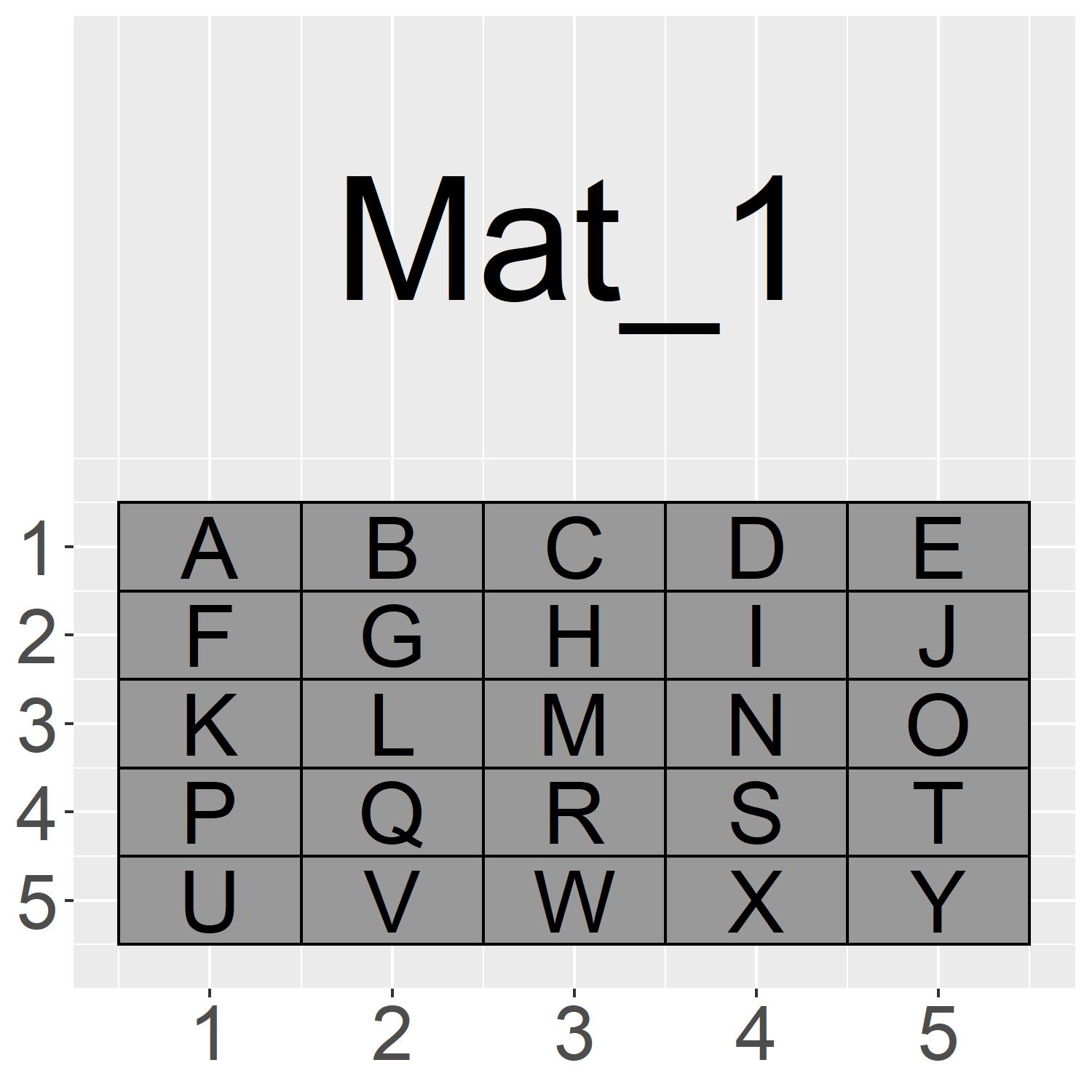
The visualisation on the left shows the matrix Mat_1. It has 5 rows (top to bottom) and 5 columns (left to right)
We can use a similar method to represent the structure of this matrix as we did for the vector. Only now we need to represent both rows and columns
To do this we use a comma “,” to separate each dimension in our square brackets “[ , ]”
The data structure of this matrix is represented as follows: \[\Large Mat\_1[1:5 , 1:5]\]

Indexing a matrix

Now we may want to extract some of the information stored inside of the Matrix.

The matrix contains letters A to Y.

The GIF on the left shows what command we would use to access each element of the matrix Mat_1
As our index now has two dimensions we need to input two different locations to find an element. We can separate these two inputs with a “,” inside of the square brackets “[ , ]”
The general rule to index a matrix is: \[\Large Mat\_1[Row , Column]\]
Note that we can select still more than one element of each dimension at a time
To select letters “G”, “H”, “I”, “L”, “M” and “N” we would use: \[\Large Mat\_1[2:3, 2:4]\]
Or we could just select letters “F”, “J”, “P” and “T” as follows: \[\Large Mat\_1[c(2, 4), c(1, 5)]\]

Play around with each of the above matrix indexing methods and make sure you understand how they work. Test yourself by writing the index to return you name!

Operators and functions covered

Base R Plot Operators and Functions Covered	Brief explanation

" <- " or " = "	Leftward assignment. This operator takes the values provided on their right and assigns them to the object on their left
" () "	Round brackets are used, as in equations, to denote operational orders ( 2 * (5 + 5) would return 20 and not 15) but they are also used to contain the inputs and arguments for function. All functions will be written as function() for this reason.
“c()”	The combine function. This function allows you to assign multiple data into many object elements at once.
“View()”	View function. This function brings up a new window to view your object. This is the neater alternative to simply viewing the object in the console.
" : "	The Range operator. The colon operator fills in all integers (whole numbers) between the initial value on its left and the final value on its right. (1:5 return 1 2 3 4 5)
“[]”	The square brackets are used to index an object. They allow you to specify which elements of the object you want to retrieve or to assign into.
“letters” and “LETTERS”	Built in alphabet vectors that can be accessed in lower case and upper case respectively.
“matrix()”	The matrix function. Used to create matrices by inputing “data” argument and its dimensions “ncol” and “nrow”. Additionally “byrow = FALSE” is the default inputting method but this can be set to TRUE if you want the data input by row instead of column.
“?” or “help()”	The function help operator. This provides a brief but detailed overview of the function, its defaults and its arguments. It sometimes contains examples.

Coming Soon

Next we will explore multi data-type objects.

These include two very important and versatile objects called lists and dataframes.

Indexing Single Datatype Objects