Logical Indexing and Debugging
Estimated Time
This lesson should take approximately 2 hours to cover and complete all the homework. Make sure you have R Studio open to work through the examples provided!
You will also be required to find some of the homework solutions yourself to get used to using Stack Overflow sites to get help
Pre-requisites
Before going through this lesson segment it is important you are already familiar with the first two parts of this lesson entitled “Indexing and Single Data-Type Objects” and Indexing and Multiple Data-Type Objects
Preamble
To round off our lesson on objects and indexing them, we will go through one of the most useful type of indexing: indexing with logicals. Remember that a logical is just a datatype of TRUEs and FALSEs. If we learn how indexing using TRUE/FALSE vectors work, then we can retrieve information from an object using a question called a conditional.
Logicals
For example “15 == 3 * 5” is asking a question of whether the left hand side is equal to the right hand side and will return a TRUE value.
15 == 3 * 5[1] TRUEWe discussed this briefly in one of the intro videos where I explained why we use the " <- " instead of " = “. The reason was that equals gets confusing because it can be” = " as a command: “make the left hand side equal to the right hand side” (leftward assignment), or it can be " == " as a question: “is the left hand side equal to the right hand side?” (conditional).
We can ask if any two strings are equal or, what is more useful, we can ask if one string is equal to any of the strings in a character vector.
"Words" == c("Words", "Unicorn", "Bicycle")[1] TRUE FALSE FALSERecycling
This illustrates an important default built into R: “Recycling”. Of course the left hand side (a character vector of length 1) isn’t actually equal to the right hand side (a character vector of length 3) but R evaluates the question element by element. Because the left hand side only has one element it recycles that element three times.
We can show how R evaluates that statement as follows
"Words" == "Words"[1] TRUE"Words" == "Unicorn"[1] FALSE"Words" == "Bicycle"[1] FALSEThe left hand side is shorter than the right hand side so it is recycled 3 times.
If we try this with a two element vector on the left hand side this pattern is more obvious:
c("Words", "Unicorn") == c("Words", "Unicorn", "Bicycle")Warning in c("Words", "Unicorn") == c("Words", "Unicorn", "Bicycle"): longer object length is
not a multiple of shorter object length[1] TRUE TRUE FALSEWe get a warning because the left hand side is not a multiple of the right hand side. This means we use the first element (“Words”) twice and the second element (“Unicorn”) only once. R allows this but warns us because it looks like a mistake.
We can replicate how R evaluates the above statment as follows:
"Words" == "Words"[1] TRUE"Unicorn" == "Unicorn"[1] TRUE"Words" == "Bicycle"[1] FALSEAs proof that that is what R is doing we can change the last element of the right hand side to “Words” to produce all TRUEs.
c("Words", "Unicorn") == c("Words", "Unicorn", "Words")Warning in c("Words", "Unicorn") == c("Words", "Unicorn", "Words"): longer object length is not
a multiple of shorter object length[1] TRUE TRUE TRUEInequalities
We can also evaluate inequalities such as less than “<” and greater than “>” as well as “<=” and “>=” for less than or equals to and greater than or equals to respectively.
15 > 3 * 5[1] FALSE15 >= 3 * 5[1] TRUE15 < 3 * 5[1] FALSEThis, of course, only applies where inequalities make sense. You should not ask if “Words” are greater than “Unicorns” but if you do R will simply look at alphabetic ordering (which comes first in the dictionary)
"Words" > "Unicorn"[1] TRUEThe Not (!) operator
The exclamation mark “!”, or not operator can be used directly in statments such as “!=” for not equals to or as a function that simply changes all TRUE to FALSE and FALSE to TRUE.
Make sure all of the below evaluations make sense.
15 != 3 * 5[1] FALSE!(15 == 3 * 5)[1] FALSE!(15 > 20)[1] TRUE!(TRUE)[1] FALSE!(c(FALSE, TRUE, FALSE))[1] TRUE FALSE TRUEIndexing with Logicals
Let’s bring back one of our objects we created in “Indexing Multiple Data-Type Objects”. We ended the lesson with a look at dataframes which we discussed can be indexed as a list (using “[[ ]]”), as a matrix (using “[ , ]”) or as named variables (using the “$”).
I’ve copied a visualisation of the object along with the code required to create it below.
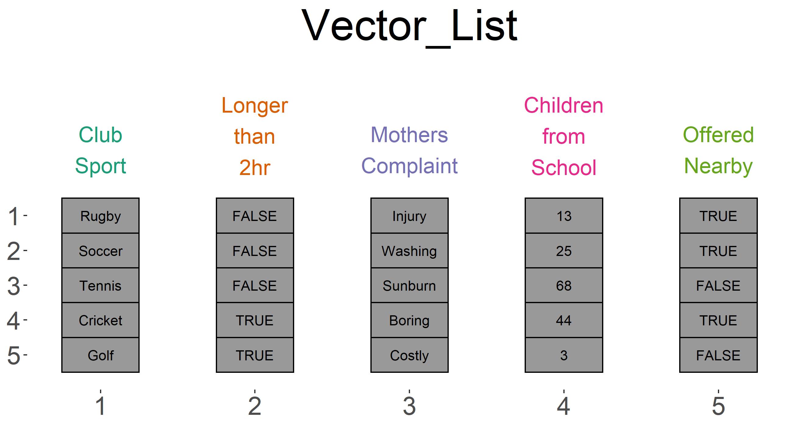
Vector_List <- list(Club_Sport = c("Rugby", "Soccer", "Tennis", "Cricket", "Golf"),
                    Longer_than_2hr = c(F, F, F, T, T),
                    Mothers_Complaint = c("Injury", "Washing", "Sunburn", "Boring", "Costly"),
                    Children_from_School = c(13, 25, 68, 44, 3),
                    Offered_Nearby = c(T, T, F, T, F))
Let’s assume we are looking to find only the sports that have at least 20 children from your kids school. We can think about this basic question more specifically by saying “return the Club_Sport variable that corresponds to the Children_from_School variable being greater than or equal to 20”. Make sure that makes sense before you proceed.
Let’s do this in steps. First, we want to evaluate which elements of the Children_from_School variable match our criteria:
Vector_List$Children_from_School >= 20[1] FALSE TRUE TRUE TRUE FALSEWe can see that the middle three observations (25, 68 and 44) are all greater than or equal to 20 because they returned TRUE.
But we want to return the names of the sports from the variable Club_Sports that correpsond to these observations. To do this we pass the logical vector directly into the vector index “Vector_List$Club_Sport”.
Vector_List$Club_Sport[c(FALSE, TRUE, TRUE, TRUE, FALSE)][1] "Soccer" "Tennis" "Cricket"Great, now we have the sports we are looking for!
We could have made this even easier by doing it in one step and asking the question directly in the index (shown below) but I wanted to show you the steps R is taking in between.
Vector_List$Club_Sport[Vector_List$Children_from_School >= 20][1] "Soccer" "Tennis" "Cricket"This is an incredibly powerful tool. It allows us to filter observations and sort through large datasets using logical questions.
Exercise
As a parent, you have the following goals:
- Avoid injury
- Don’t watch a boring sport for more than two hours
- Have no more than 30 children from your childs school at the club
Use conditional indexing to to return the sports that match the above criteria. (hint: you can use th “&” operator to combine conditional statements together)
Indexing by Exclusion and an Intro to Debugging
Let’s start by creating a simple object that contains the numbers 1 to 10.
object_1 <- LETTERS[1:10]
object_1
[1] "A" "B" "C" "D" "E" "F" "G" "H" "I" "J"If we want to see the last 5 letters we could simply ask for the vector to return elements 6 to 10, or we could ask for the vector to return all elements except elements 1 to 5.
To exclude elements from a vector we use the “-” operator.
These should be equivalent.
object_1[6:10][1] "F" "G" "H" "I" "J"object_1[-(1:5)][1] "F" "G" "H" "I" "J"Notice that we needed to put parentheses “()” around the 1:5 otherwise it would only make the 1 negative and we would be asking the vector to return all elements from -1 (which doesn’t exist until 5).
As we saw earlier, we can also use conditional indexing to return what we want.
To get elements 6 to 10, we could ask for the vector to return the elements from 1 to 10 that are greater than 5.
object_1[1:10 > 5][1] "F" "G" "H" "I" "J"Alternatively we could use the not “!” operator and return all elements from 1 to 10 that are not less than 6.
object_1[!(1:10 < 6)][1] "F" "G" "H" "I" "J"This is very useful in many scenarios but what happens if we mix up the negative operator “-” with the not operator“!”?
Let’s see if they are equivalent and what would happen:
object_1[!(1:5)]character(0)Using the not operator “!”, which is designed for data type logical on data type numeric returns nothing (but not an error?).
object_1[-(1:10 < 6)][1] "B" "C" "D" "E" "F" "G" "H" "I" "J"Using a negative operator “-”, which is designed for data type numeric on data type logical produces letters “B” to “J”???
This is the type of confusing results which makes you want to give up on silly languages like R? I’ve often secretly thought my machine was broken or that I discovered a bug when I see weird results like this.
Instead of giving up we should try to follow a consistent method of debugging errors and finding where our logic breaks down.
Let’s go through the problem above using these steps and it might explain both results.
Step 1 - Create a simplified reproducible example of your data
If you have a table with 1000 rows and 25 columns of proprietary data, create a mini version of simulated data with 5 rows and 3 columns.
It is easier to see what is going wrong on fewer data, and simulating the data makes it simpler to share your problem with an online community. Additionally, simulating the problem into its smllest form forces you to generalise your procedure and separate the problem from everything else.
In our example the data we’re working with is simple enough and the data is already simulated (ie anyone can type “object_1 <- LETTERS[1:10]” and create our data wbecause “LETTERS” is a built in, common, dataset).
Step 2 - Seperate every underlying step of the procedure into its simplist parts
Our code looks as follows:
object_1[-(1:10 < 6)][1] "B" "C" "D" "E" "F" "G" "H" "I" "J"We can identify three basic parts to this.
- The index vector “object_2 > 5”
- The exclude operator “-”
- The object “object_2”
Step 3 - Analyse each step in the order in which R processes them
R, maths and most programming languages work work from the inside out. This means when you say “object_1[-(1:10 < 6)]”, R starts by solving the inner most bracket “1:10 < 6”, then applies the negative “-”, then uses this to index the object on the outside.
Let’s do these steps ourselves. Taking the result of each step and using it for the following step. This will allow us to see where we are getting the unexpected result
Step (1)
1:10 < 6 [1] TRUE TRUE TRUE TRUE TRUE FALSE FALSE FALSE FALSE FALSEStep (2)
-c(TRUE, TRUE, TRUE, TRUE, TRUE, FALSE, FALSE, FALSE, FALSE, FALSE) [1] -1 -1 -1 -1 -1 0 0 0 0 0We can see here the beginnings of why we’re getting a weird result.
The negative operator “-” only deals with numerical data. When we give it logical data, it coerces it into numerical with TRUE = 1 and FALSE = 0.
It then applies the negative to these numbers.
Now we can try to predict what will happen next. Think about our negative indexing we looked at earlier.
We should see the “-1” index return everything except the first element. Repeating the same index position or indexing position “0” has no effect so we simply get the full vector except for the first element returned to us.
object_1[c(-1, -1, -1, -1, -1, 0, 0, 0, 0, 0)][1] "B" "C" "D" "E" "F" "G" "H" "I" "J"Mystery solved!
Try remember these three steps when you run into confusing results. You often end up solving the problem by step one or two.
(1) Create a simplified reproducible example of your data
(2) Seperate every underlying step of the procedure into its simplist parts
(3) Analyse each step in the order in which R processes them
I find this very useful so I hope it helps.
Homework
Using the built in dataset “airquality”, calculate the average temperature for each of the 5 months.
- Hint use “datasets::” to access the built in datasets, the function “mean()” to calculate averages and add the argument “na.rm = T” to your function if you want the answer to remove NA values.
plot each of these average in a column chart (use the function “barplot()” and “?” to learn more about “barplot”)
plot the median for each month (y axis) against the mean for each month (x axis). Then add a straight line 1:1 relationship to your graph (45 degree line where change in X = change in Y).
Thinking back to 1st year stats, what would it mean about the distribution of tempertaures if most of the points where below the line or above the line?
Lastly, using instructions from this post, create a histrgam of the temperature from all months. Then, using this Stack Overflow post, overlay the density function of a normal distribution.
- Hint: make sure you set “freq = F” or “prob = T” in your histogram otherwise you won’t be able to see your density function.
How would you characterise the distribution of temperature?
swirl homework
Open swirl (remember you need to call it from the library using library(swirl) each time you open R Studio and then initialise a swirl session using swirl()).
Select “R Programming” and complete the lessons names “Logic” and “Base Graphics”
Operators and functions covered
| Base R Plot Operators and Functions Covered | Brief explanation |
|---|---|
| “+” | Addition |
| "*" | Multiplication |
| “/” | Division |
| “:” | Generates a range from the left hand side to the right hand side. 3:6 = c(3, 4, 5, 6) |
| “>” | Greater than |
| “<” | Less than |
| “>=” | Greater than or equals to |
| “<=” | Less than or equals to |
| “!” | The not operator. Can be combined with other inequalities such as “!=” not equals to or “!<”, or it can be used as a function on a vector of logicals “!()” |
| “-” | Two uses: either subtraction or exclusion. Exclusion works like a normal index call except instead of calling element “[1]”, it will return everything except element 1 “[-1]” |
| “datasets::” | datasets and the :: operator. These are often used in conjuction to gain access to the built in R datasets. They are a great set of data to use as reproducible examples because everyone has access to them. The :: operator just allows you to access a package in your library even if it hasn’t been called using library (try “swirl::swirl()”) |
Coming Soon
In our next batch of lessons we will go through loops and custom functions. These allow you to make generic instructions that can be passed on to many different datasets instead of writing out similar functions over and over again.
Think about your homework example where you calculated the mean temperature for every month. Surely there is an easier way than writing out almost identical statements for each month? That’s what we will learn next!