Indexing Multiple Datatype Objects
Estimated Time
This is quite a long lesson should take approximately 3 hours to cover and complete all the homework. Make sure you have R Studio open to work through the examples provided!
You will also be required to find some of the homework solutions yourself to get used to the R Q&A forums
Pre-requisites
Before going through this lesson segment it is important you are already familiar with the first half of this lesson entitled “Indexing and Single Data-Type Objects”
Recap and Coercion of DataTypes
Checking DataTypes
All objects previously covered (Vectors and Matrices) as well as higher dimensional objects (Arrays) require that all information contained in them are of the same data type. A quick recap of the 4 basic data types are given below:
Character (this contains “string” data like words or letters)
Numeric or Double (these are numbers). Note that Integer is another data type for whole numbers
Logical (these are TRUE or FALSE and can be abbreviated to T and F)
Factor (a special data type used for categories)
To check whether data is of a specific type we can use the prefix “is.numeric()” or “is.logical()” etc…
is.logical(TRUE)[1] TRUEis.numeric(45)[1] TRUEis.factor("category")[1] FALSEPlay around with this using different inputs to get an understanding of how data is categorised.
Instead of asking if some data is each of the various data types, we could instead simply ask what data type it is using the function “typeof()”
typeof(45)[1] "double"typeof(T)[1] "logical"typeof("T")[1] "character"Notice how the "" will make R read the T as a character instead of a logical.
Assigning DataTypes (Coercion)
We can also coerce something into a specific data type (where possible) using the function “as.character()”, “as.logical()”, “as.factor()” etc…
as.character(45)[1] "45"as.numeric("45")[1] 45as.factor("category")[1] category
Levels: categorySome of these are trivial and obvious like the examples above.
Below are some less obvious coercions that illustrate how R naturally converts certain data:
as.logical(c(0, 1, 0))[1] FALSE TRUE FALSEas.numeric(c(FALSE, TRUE, FALSE))[1] 0 1 0Here we can see that R coerces TRUE and FALSE into 1 and 0 respectively. This can happen when we ask R to coerce something but it can also be done by R automatically.
Automatic Coercion
R is considered a high level programming language which means that it can interpret certain things on your behalf.
For example, as we saw in the previous lesson, you are required to create an object and designate what type of data it will contain before assigning any information to it. R will assume that your object is of type “numeric” if you want to put a number inside it and assume it is of type “character” if you want to put a word inside it.
This makes things a lot simpler to write. Consider the below example of what we may have needed to specify first in order to do the simple task of assigning the number 42 into an object called “object_1”:
object_1 <- vector(mode = "numeric", length = 1)
object_1[1] <- 42
Instead of just:
object_1 <- 42This is very convenient but it can also lead to problems when R makes assumptions on your behalf.
Take the example of adding a single string to a vector of numbers:
c(42, 58, "32", 65)[1] "42" "58" "32" "65"R coerces all of your numbers to characters without producing an error or a warning.
This means we need to understand how R makes these decisions in order to make the “debugging” process simpler.
Some Basic R Coercion Rules
These are the basic rules I’ve come across regarding R’s automatic coercion.
When in doubt convert all vectors to character
If you have logical mixed with numbers it will convert the logical to numeric
When R cannot coerce the data it produces an NA in the place of the failed to coerce element (NA, NULL, NaN and Inf are explained in more detail in this blog post) - Fortunately it will give you a warning message.
Convert all dataframe “strings” to factor (not character). We will explain dataframes and factors later in this lesson
Multiple Data-Type Objects
There is only really one type of object that can contain more than one datatype. That is a list. Lists are highly versatile one dimensional objects.
By highly versatile we mean they can contain anything we want: different data types, entire vectors or matrices, other lists with lists inside each of those lists etc…
But before we see all of the exciting things lists can do, let’s just start with a simple 5 element list that contains different datatypes.
List of Elements
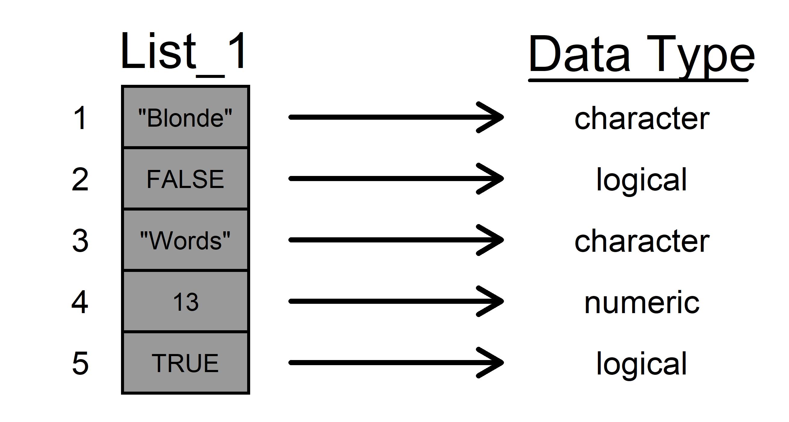
The list (“List_1”) visualised on the left has length 5 and it is made up of factor, logical, character and, numeric data
To create this object:
List_1 <- list("Blonde", FALSE, "Words", 13, TRUE)- Lists can be indexed as follows (notice the double square brackets):
\[\Large List\_1 [[ element ]]\]
Visualising List Indexing and Datatype Queries
Let’s see what indexing the elements of that list looks like as well as double checking that the data is really made up of different datatypes.
List of Matrices
OK so far lists just look like vectors that can hold different datatypes. What else can they do?
Lists are extremely versatile because they can also hold different data structures. Next we’re going to show how we can make a list of two matrices.
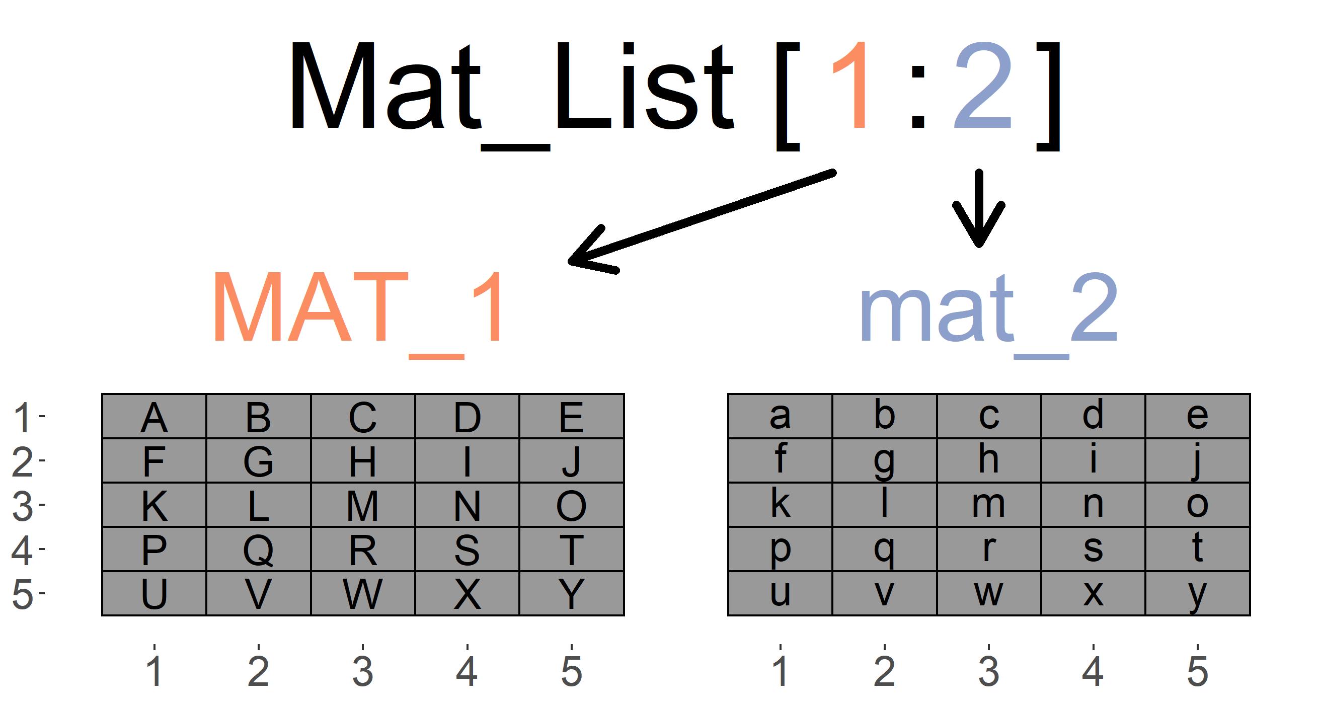
The list (“Mat_List”) visualised on the left has length 2 and it is made up of 2 5x5 Matrices (Note that we have also assigned names to each element of our list).
To create this object:
Mat_List <- list(MAT_1 = matrix(LETTERS[1:25], nrow = 5, byrow = T), mat_2 = matrix(letters[1:25], nrow = 5, byrow = T))Names can also be given to elements of a vector. To access the names attribute simple type “names(object)” for example:
names(Mat_List)[1] "MAT_1" "mat_2"Or to assign names to the object:
names(Mat_List) <- c("MAT_1", "mat_2")
Try this out yourself.
Visualising and Indexing a List of Matrices
We can now index both the list element as a whole (ie each matrix), or we can index elements within each list element (ie the letters within each matrix)
The above animations show off the versatility of lists (they can hold pretty much anything) but they don’t look very elegant. Next we will look at a special case where we have a list of vectors of equal length (also known as a dataframe).
Dataframes will be the most important datatype you will work with so its important you understand exactly what it is.
List of Vectors and Dataframes
The last example of a list that we will look at is by far the most important. It is simply a list of equal length vectors.
An Example
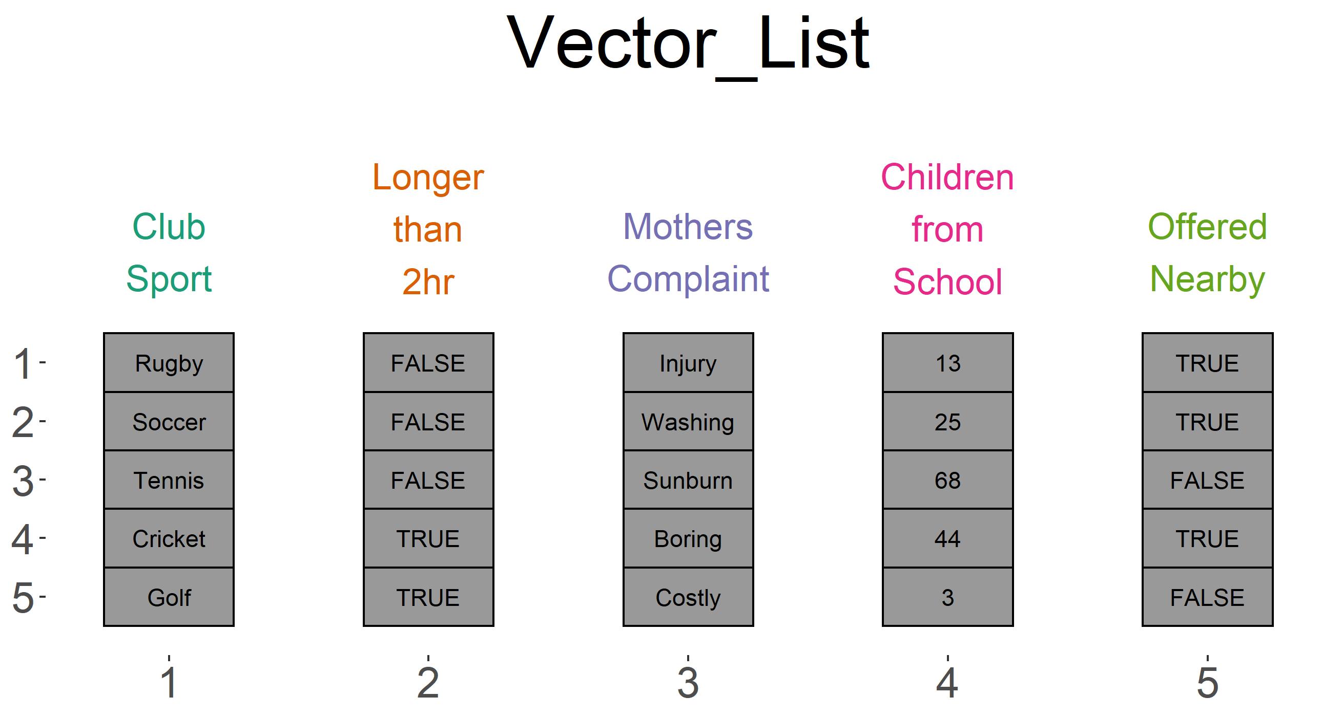
Because this data structure is so important, it deserves its own example. Let’s assume you are a mother trying to decide which after school sports club to enroll your child in. You have gained access to a survey conducted by a parents organisation from the previous year and have narrowed the survey down to 5 variables you think will be important.
ClubSport (vector indicating which sport is offered by the club)
Longerthan2hr (vector indicating whether the sport can sometimes go over 2 hours)
MothersComplaint (vector of specifying the key words of most mothers complaints about the sport)
ChildrenfromSchool (vector that counts the number of children at the each club that attend the saem school as your child)
OfferedNearby (vector that you created that specifies whether the club is nearby your house)
You can create this list yourself as follows:
Vector_List <- list(Club_Sport = c("Rugby", "Soccer", "Tennis", "Cricket", "Golf"),
                    Longer_than_2hr = c(F, F, F, T, T),
                    Mothers_Complaint = c("Injury", "Washing", "Sunburn", "Boring", "Costly"),
                    Children_from_School = c(13, 25, 68, 44, 3),
                    Offered_Nearby = c(T, T, F, T, F))
The datatype for each element of this list is character, logical, character, double, logical respectively. Test this out using typeof() on each element of your list.
The data can be seen as a list of vectors and is visualised below.
Note however that these vectors are related to each other
The first element of each vector relates to the first club, the second element relates to the second club and so on…
This means we can think of each row as an observation and each column as a variable.
Going from List of Vectors to a Dataframe
Because each vector is related to each other where each row is made up of data points of the same observation, it is appropriate to designate the list of vectors as a dataframe.
We can do this as follows:
Vector_List <- as.data.frame(Vector_List)This allows us to index the object in three different ways.
- First and foremost a vector is a list and can be indexed as:
\(Vector\_List [[ element ]]\)
- Second, this dataframe has named columns so we can index each named column (vector) using the $ operator
\(Vector\_List\$Variable Name\)
- Third, we can index a dataframe as if it were a two dimensional matrix
\(Vector\_List[row , column]\)
We can see all three indexing methods below
Visualising and Indexing a Dataframe
Homework
Create an object called “homework_1” that is a frame with 100 rows and 3 columns.
Make the first variable name “Unique_Identifier” and populate it with any characters so long as none of them repeat
Make the second column a variable named “Hours_Studied_Per_Semester” and populate it with numbers that start from 3 and increases in increments of 3 until they reach 300 (Hint use the function called “seq” to produce sequences).
- Remember ?“function name” for help or example(“function name”). Try “?seq”
- Make the third variable name “Marks” a fill it with numbers that are have a mean equal to the 15% + (10 * hours studied per semester)^0.5 and add an error term that follows a normal distribution with a mean of 0% and std deviation of 5% (google “R random number generating” to help with this)
- If you have any values that are above 100%, limit them to 100%.
Plot your data so that it is clear what the relationship between hours studied and amrks is. (Again google some basic plots - nothing too fancy we will go over plotting later)
SWIRL
- Complete swirl R programming lesson 1 - 7.
To do this execute the following commands:
install.packages("swirl")This function searches the CRAN repository for a package called swirl and downloads it. Once the download is complete it will be added to your library of packages, viewable in the bottom right pane under “Packages”.
You only need to downlaod a package once per machine that you use.
All of the packages are in your library but not necessarily called to the environment.
If a package is called to the environment it will have a tick next to it.
To activate a package in your library in an R script type:
library(swirl)You will need to call the package from your library every session that you use it. To get started with the lesson
swirl()Type your name or nickname into the console.
Select the option for “R Programming”
Select the option for “Basic Building Blocks” (continue until you have completed up to and including “Matrices and Data Frames”)
Remember to ask questions and have in in R!
Operators and functions covered
| Base R Plot Operators and Functions Covered | Brief explanation |
|---|---|
| " is.character() " " is.logical() " etc… | Data type conditional. These functions evaluate whether an object is a particular datatype and return TRUE/FALSE accordingly |
| " typeof " | Data type query Asks what data type an object is. Returns the object type as a character string |
| " as.numeric() " " as.factor " | The coerce function. This function allows you to coerce an object into a datatype of your choice. Some coercion is not possible and will return “NA” when the function fails. Note you can also coerce into a dataframe using “as.data.frame()” |
| “list()” | List function. This function is used to create a list. You may name any elements within the “()” and separate each list element with a “,” |
| " [[]] " | The list index operator. The double square brackets accesses any information with a particular list element. The normal single square brackets “[]” are used to subset a list (it will still return a list though) |
| “names()” | The names function provides access to the names attribute of an object. Vectors, lists and dataframes can all have names assigned to their elements. |
Coming Soon
In our next lesson we will go through Conditional statements as a form of indexing using logicals. Additionally, we will introduce operational ordering to explain how R reads your instructions.
There will also be a short introduction to how to debug your code.